第四章 Two-Player Zero-Sum Game

[TOC]

4.1 定义

A two-player zero-sum game is a strategy game $ G = \{ \{ 1, 2 \}, \{ A_1, A_2 \}, \{ u_1, u_2 \} \} $ such that

$$u_1(a_1, a_2) + u_2(a_1, a_2) = 0 \quad \text{for } a_1 \in A_1 \text{ and } a_2 \in A_2.$$

One player wins while the other losses

4.1.1 举例

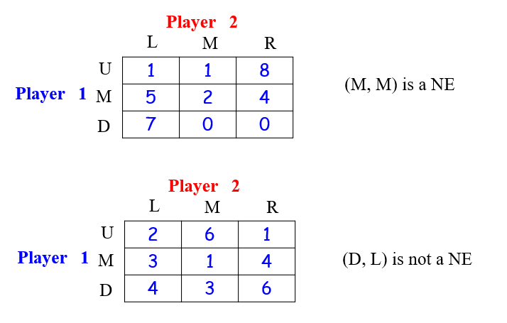
• 对于两人的零和博弈，约定考虑第一个人的收益矩阵，缩略图如下

• $ u(a_1, a_2)$即为第一个人的收益矩阵

4.1.2 Maxmin (最大化最小原则例子)

Player 1 method: $\max_{a_1 \in A_1} \min_{a_2 \in A_2} \, u(a_1, a_2)$

Player 1 selects M: $ M \in \arg\max_{a_1 \in A_1} \min_{a_2 \in A_2} u(a_1, a_2) $

• $a_1=U$ ，$a_2$会最小化收益，因此收益1
• $a_1=M$ ，$a_2$会最小化收益，因此选择2
• $a_1=D$ ，$a_2$会最小化收益，因此选择0

最大化选择，因此选择M

Player 2 method: $ \max_{a_2 \in A_2} \min_{a_1 \in A_1} \, u_2(a_1, a_2)$

Player 2 selects M

• 在这个情况下，Player 2的收益矩阵相当于Player 1的收益矩阵全部取负值
• $a_2=L$ ，$a_1$会最小化收益，因此收益-7
• $a_2=M$ ，$a_1$会最小化收益，因此选择-2
• $a_2=R$ ，$a_1$会最小化收益，因此选择-8

最大化选择，因此选择M

4.2 Minmax (最小化最大原则)

Player 2 method: $ \max_{a_2 \in A_2} \min_{a_1 \in A_1} u_2(a_1, a_2) $

From $ u_2(a_1, a_2) = -u(a_1, a_2) $, we have

$ \max_{a_2 \in A_2} \min_{a_1 \in A_1} u_2(a_1, a_2) = \max_{a_2 \in A_2} \min_{a_1 \in A_1} (-u(a_1, a_2)) $

By $ \max(-f(x)) = -\min(f(x)) $, we get

$ \max_{a_2 \in A_2} \min_{a_1 \in A_1} u_2(a_1, a_2) = -\min_{a_2 \in A_2} \max_{a_1 \in A_1} u(a_1, a_2) $

Player 2 method: $ \arg\min_{a_2 \in A_2} \max_{a_1 \in A_1} u(a_1, a_2) $

4.2.1 例1

还是上文的例子：Player 2 method: $ \min_{a_2 \in A_2} \max_{a_1 \in A_1} \, u_2(a_1, a_2)$

• $a_2=L$ ，$a_1$会最大化收益，因此收益7
• $a_2=M$ ，$a_1$会最大化收益，因此选择2
• $a_2=R$ ，$a_1$会最大化收益，因此选择8

最小化选择，因此仍旧选择M

在这里我们发现两个player的选择：

$ \min_{a_2 \in A_2} \max_{a_1 \in A_1} \, u_2(a_1, a_2)$=$\max_{a_1 \in A_1} \min_{a_2 \in A_2} \, u(a_1, a_2)$

4.2.2 例2

$ \min_{a_2 \in A_2} \max_{a_1 \in A_1} \, u_2(a_1, a_2)$>$\max_{a_1 \in A_1} \min_{a_2 \in A_2} \, u(a_1, a_2)$

• Player 1:3
• Player 2:4

4.2.3 MinMax ≥ MaxMin

Lemma: For a two-player zero-sum finite game $ G $, we have

$$\min_{a_2 \in A_2} \max_{a_1 \in A_1} u(a_1, a_2) \geq \max_{a_1 \in A_1} \min_{a_2 \in A_2} u(a_1, a_2)$$

Proof: For any function $ F(x, y) $, we have

$$F(x, y) \geq \min_y F(x, y) \quad \text{for any } y$$ $$\max_x F(x, y) \geq \max_x \min_y F(x, y) \quad \text{for any } x$$ $$\min_y \max_x F(x, y) \geq \max_x \min_y F(x, y)$$

• 实际上对于任何一个问题都有minmax$\geq$maxmin

4.3 Two-Players Zero-Sum Nash Equilibrium

Theorem: For a two-player zero-sum finite game $ G = \{ \{1, 2\}, \{A_1, A_2\}, u \} $, let player 1 select

$$a_1^* \in \arg\max_{a_1 \in A_1} \min_{a_2 \in A_2} u(a_1, a_2),$$

and let player 2 select

$$a_2^* \in \arg\min_{a_2 \in A_2} \max_{a_1 \in A_1} u(a_1, a_2).$$

The strategy outcome $(a_1^, a_2^)$ is a Nash Equilibrium if and only if

$$\max_{a_1 \in A_1} \min_{a_2 \in A_2} u(a_1, a_2) = \min_{a_2 \in A_2} \max_{a_1 \in A_1} u(a_1, a_2).$$

4.3.1 Proof

Necessity:

要证明：

If $(a_1^, a_2^)$ is a NE, then

$$u_1(a_1^*, a_2^*) \geq u_1(a_1, a_2^*) \text{ for all } a_1 \in A_1,$$ $$u_2(a_1^*, a_2^*) \geq u_2(a_1^*, a_2) \text{ for all } a_2 \in A_2.$$

By using $u_1(\cdot, \cdot) = u(\cdot, \cdot)$ and $u_2(\cdot, \cdot) = -u(\cdot, \cdot)$, we have

$$(a_1^*, a_2^*) \text{ is a NE} \iff u(a_1, a_2^*) \leq u(a_1^*, a_2^*) \leq u(a_1^*, a_2)$$ $$\iff u(a_1, a_2^*) \leq u(a_1^*, a_2).$$

If $(a_1^, a_2^)$ is a NE, then we have

$$u(a_1, a_2^*) \leq u(a_1^*, a_2) \rightarrow \max_{a_1} u(a_1, a_2^*) \leq \min_{a_2} u(a_1^*, a_2),$$ $$a_2^* \in \arg \min_{a_2 \in A_2} \max_{a_1 \in A_1} u(a_1, a_2), \quad a_1^* \in \arg \max_{a_1 \in A_1} \min_{a_2 \in A_2} u(a_1, a_2).$$

Therefore,$\min_{a_2 \in A_2} \max_{a_1 \in A_1} u(a_1, a_2) \leq \max_{a_1 \in A_1} \min_{a_2 \in A_2} u(a_1, a_2).$

结合$\min_{a_2 \in A_2} \max_{a_1 \in A_1} u(a_1, a_2) \geq \max_{a_1 \in A_1} \min_{a_2 \in A_2} u(a_1, a_2)$

即可得到相等结果

Sufficiency:

要证明：

If $ \min_{a_2 \in A_2} \max_{a_1 \in A_1} u(a_1, a_2) = \max_{a_1 \in A_1} \min_{a_2 \in A_2} u(a_1, a_2), $=
then =$ u(a_1, a_2^) \leq u(a_1^, a_2). $

We have

$$u(a_1, a_2^*) \leq \max_{a_1} u(a_1, a_2^*) = \min_{a_2 \in A_2} \max_{a_1 \in A_1} u(a_1, a_2),$$

and

$$u(a_1^*, a_2) \geq \min_{a_2} u(a_1^*, a_2) = \max_{a_1} \min_{a_2} u(a_1, a_2).$$

Thus , $ u(a_1, a_2^) \leq u(a_1^, a_2)$, $(a_1^, a_2^)$ is a NE

4.3.2 Find Nash Equilibrium

4.4 Mixed strategy

Strategic game
$N = \{1, 2\}$
$A_1 = {a_1, a_2, \dots, a_m}$, $A_2 = {b_1, b_2, \dots, b_n}$
$u_1 (a_i, b_j) = u(a_i, b_j) = u_{ij}$, $M = (u_{ij})_{m \times n}$

Mixed strategy
$p = (p_1, p_2, \dots, p_m) \in \Delta_1$ is a mixed strategy over $A_1$
$q = (q_1, q_2, \dots, q_n) \in \Delta_2$ is a mixed strategy over $A_2$

The expected payoff for player 1 on mixed outcome $(p, q)$
$U(p, q) = \sum_{i, j} p_i q_j u(a_i, b_j) = \sum_{i, j} p_i q_j u_{ij} = p M q^{\top}$

Player 1’s methods:
$\max_{p \in \Delta_1} \min_{q \in \Delta_2} U_1(p, q) = \max_{p \in \Delta_1} \min_{q \in \Delta_2} p M q^{\top}$

Player 2’s methods:
$\max_{q \in \Delta_2} \min_{p \in \Delta_1} U_2(p, q) = \min_{q \in \Delta_2} \max_{p \in \Delta_1} p M q^{\top}$

Lemma
We have $\max_{p \in \Delta_1} \min_{q \in \Delta_2} U(p, q) \leq \min_{q \in \Delta_2} \max_{p \in \Delta_1} U(p, q)$

4.4.1 混合策略零和博弈的纳什均衡

Theorem:
For a two-player zero-sum finite game $G = \{ \{1, 2\}, \{A_1, A_2\}, u \}$, let player 1 select

$$p^* \in \arg \max_{p \in \Delta_1} \min_{q \in \Delta_2} U(p, q),$$

and let player 2 select

$$q^* \in \arg \min_{q \in \Delta_2} \max_{p \in \Delta_1} U(p, q).$$

The mixed strategy outcome $(p^, q^)$ is a Mixed Strategy Nash Equilibrium (MNE) if and only if

$\max_{p \in \Delta_1} \min_{q \in \Delta_2} U(p, q) = \min_{q \in \Delta_2} \max_{p \in \Delta_1} U(p, q).$

Proof

1. Maximization by Player 1: Player 1 seeks to maximize their minimum payoff by choosing a mixed strategy $p \in \Delta_1$. This means player 1 will select $p^* \in \arg \max_{p \in \Delta_1} \min_{q \in \Delta_2} p M q^\top$.

   The objective is:

   $\max_{p \in \Delta_1} \min_{q \in \Delta_2} p M q^\top.$

   This represents the maximum of the minimum payoff player 1 can secure, considering that player 2 is choosing their strategy qq to minimize player 1’s payoff.

2. Minimization by Player 2: Similarly, player 2 aims to minimize their maximum loss, selecting $q^* \in \arg \min_{q \in \Delta_2} \max_{p \in \Delta_1} p M q^\top$.

   The objective is:

   $\min_{q \in \Delta_2} \max_{p \in \Delta_1} p M q^\top$.

   This represents the minimum of the maximum payoff player 2 has to endure, considering that player 1 is choosing their strategy pp to maximize their payoff.

3. The Minimax Theorem: By the minimax theorem for zero-sum games, we know that the optimal strategies $p^ $and $q^$ for players 1 and 2, respectively, will lead to the following equality:

   $\max_{p \in \Delta_1} \min_{q \in \Delta_2} p M q^\top = \min_{q \in \Delta_2} \max_{p \in \Delta_1} p M q^\top$.

   This is the core of the minimax theorem, which ensures that the game has an equilibrium point in mixed strategies where both players are choosing their strategies optimally.

4. Conclusion: Since $p^$ and $q^$ satisfy the conditions of the minimax theorem, we conclude that the outcome of the game (given by $p^, q^$) will be a Mixed Strategy Nash Equilibrium (MNE). The equality

   $\max_{p \in \Delta_1} \min_{q \in \Delta_2} p M q^\top = \min_{q \in \Delta_2} \max_{p \in \Delta_1} p M q^\top$

   holds true, confirming that the mixed strategy outcome $(p^, q^)$ is indeed a Nash equilibrium.

4.4.2 General John von Neumann’s minimax theorem

The Minimax Theorem:

Let $X \subset \mathbb{R}^n$ and $Y \subset \mathbb{R}^m$ be compact convex sets.

If $f: X \times Y \to \mathbb{R}$ is a continuous function such that:

• $f(\cdot, y): X \to \mathbb{R}$ is concave for fixed $y$;
• $f(x, \cdot): Y \to \mathbb{R}$ is convex for fixed $x$,

then we have:

$$\max_{x \in X} \min_{y \in Y} f(x, y) = \min_{y \in Y} \max_{x \in X} f(x, y).$$

4.4.3 John von Neumann’s Minimax Theorem (1928)

The Minimax Theorem: For a two-player zero-sum finite game $G = \{ \{1, 2\}, \{A_1, A_2\}, u \}$, we have:

$$\max_{p \in \Delta_1} \min_{q \in \Delta_2} p M q^{\top} = \min_{q \in \Delta_2} \max_{p \in \Delta_1} p M q^{\top}.$$

Corollary: Two-person finite zero-sum games have at least one mixed-strategy Nash equilibrium: any pair of optimal strategies is a Nash equilibrium.

4.4.4 Example

Player 1’s mixed strategy: $(x_1, x_2)$

$U_2 (L) = -3x_1 + 2x_2, \quad U_2 (R) = x_1 - x_2$

The optimal solution for Player 2 is:
$\max(-3x_1 + 2x_2, x_1 - x_2)$

The payoffs for Player 1 is:
$-\max(-3x_1 + 2x_2, x_1 - x_2) = \min(3x_1 - 2x_2, -x_1 + x_2)$

The solution for Player 1 is:
$(x_1, x_2) \in \arg\max_{(x_1, x_2)} \min(3x_1 - 2x_2, -x_1 + x_2)$

This is equivalent to:(Linear programming)

$$\begin{align} \max \quad&v \\ \text{s.t.}\quad &3x_1 - 2x_2 \geq v, \\ &-x_1 + x_2 \geq v, \\ &x_1 + x_2 = 1, x_1 > 0, x_2 > 0 \end{align}$$

4.4.5 Theorem

The optimization problem of

$\max_{p \in \Delta_1} \min_{q \in \Delta_2} p M q^{\top}$

is equivalent to:

$$\begin{align} \max \quad&v \\\text{s.t.} \quad& p M \geq v \mathbf{1}, \\& p = (p_1, \dots, p_m) \in \Delta_1, \quad \\&\mathbf{1} = (1, \dots, 1)^{\top} \end{align}$$

Linear programming:Can be solved in polynomial time.

4.6 Symmetric Game for 2-player Zero-sum

$N = \{1,2\} , A_1 = \{a_1, a_2, \dots, a_n\} , A_2 = \{b_1, b_2, \dots, b_n\}$
$u_1(a_i, b_j) = u_{ij}, \quad M = (u_{ij})_{n \times n}, \quad M = -M^{\top}$

Theorem: For a symmetric game , we have :

$$\max_{p \in \Delta_1} \min_{q \in \Delta_2} p M q^{\top} = \min_{q \in \Delta_2} \max_{p \in \Delta_1} p M q^{\top} = 0$$

Proof:

$$\max_{p \in \Delta_1} \min_{q \in \Delta_2} p M q^\top \geq \min_{q \in \Delta_2} q M q^\top = 0$$ $$\min_{q \in \Delta_2} \max_{p \in \Delta_1} p M q^\top \leq \max_{p \in \Delta_1} p M p^\top = 0$$

Or?:

$$\max_{p \in \Delta_1} \min_{q \in \Delta_2} p M q^\top \leq \max_{p \in \Delta_1} p M p^\top = 0$$ $$\min_{q \in \Delta_2} \max_{p \in \Delta_1} p M q^\top \geq \min_{q \in \Delta_2} q M q^\top = 0$$

4.7 How to find Nash Equilibria

• Calculate directly
  • find the best response functions
  • calculate Nash equilibria
• Eliminate all dominated strategy
• For two-player zero-sum player, linear programming